A hypothesis test asks whether a sample fits a claim about a population. The claim gives a model, for example “70% of the seeds germinate”, so we know which samples to expect. A sample always differs a little from the truth, so the real question is how far is “too far”.
Example
A supplier claims that 70% of its seeds germinate. In a sample of 20, 10 germinate: p^=10/20=0.5. But 20 good seeds would not give exactly 20⋅0.7=14 either. Is 10 too few?
Definition
What the claim predicts: the null distribution
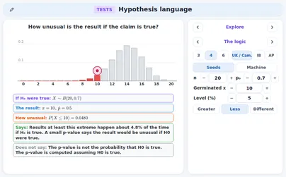
The claim to be tested is the null hypothesisH0. If H0 holds, the count follows a known law, the null distribution: here X∼B(20,0.7) for the number of seeds that germinate. It shows what chance alone does when the claim is right.
Example
Under H0 the mean is 14 and the standard deviation 4.2≈2.0494. The most likely count is 14, P(X=14)≈0.1916. A count of 10 is about 2 standard deviations below the mean.
Rule
How unusual is the result?
One result is always unlikely, so we ask for the probability of a result at least as extreme: as far from what H0 expects, or farther, in the direction that doubts the claim. If it is small, the result would be unusual when the claim is right.
Example
For 10 germinated seeds the doubt goes downwards: P(X≤10)=0.0480 (calculator: binomcdf(20, 0.7, 10)). Results at least this extreme happen about 4.8% of the time if H0 is true.
Definition
The p-value
The p-value is the probability, assuming H0 is true, of a result at least as extreme as the observed one. It is worked out inside the null distribution and lies between 0 and 1: the smaller it is, the stronger the evidence against H0.
Example
The seeds: p=P(X≤10)=0.0480, the total height of the shaded bars 0 to 10. In words: if H0 is true, results at least as extreme as 10 germinated seeds happen about 4.8% of the time.
Rule
H0 and H1 from a claim in words
A claim about a parameter (a population share p or mean μ, never the sample value p^ or xˉ) becomes two statements. H0 holds the equality: p=p0 or μ=μ0. H1 is what the test looks for: >, < or =, never =. Choose H1 from the question, before looking at the data.
Example
“A supplier says 70% of the seeds germinate; a grower thinks fewer.” H0:p=0.7, H1:p<0.7.“Is the machine off the 500 ml target?” H0:μ=500, H1:μ=500.“Are deliveries slower after the change?” With μd the mean of after minus before: H0:μd=0, H1:μd>0.
Rule
One-sided or two-sided
If H1 names a direction (> or <) the test is one-tailed: one end of the null distribution counts. If H1 says “different” (=) it is two-tailed: both ends count, and for a symmetric curve the p-value is twice the one-sided one. The direction comes from the question, never from the data.
Example
A statistic z=1.8. One-sided: P(Z>1.8)=0.0359. Two-sided: 2⋅0.0359=0.0719. At 5% the one-sided test rejects H0 and the two-sided one does not, so H1 must be chosen before the data are seen.
Definition
The significance level
The significance levelα is chosen before the test, often 5% or 1%. It is the probability of rejecting H0 when H0 is true: a wrong rejection, the Type I error. With α=0.05 about 1 test in 20 rejects a true H0. The p-value belongs to the sample; the level is fixed beforehand.
Example
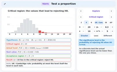
The rule “reject H0 if 10 or more of 20 parcels are late” has, when H0: p=0.3 is true, probability P(X≥10)=0.0480 of rejecting. So in 1000 honest checks about 48 would wrongly reject: 0.0480 is the actual level of the rule.
Rule
Tails and the critical value
For a normal statistic the critical value cuts off the tail with area α. One-tailed: the whole level in one tail, z=1.645 at 5%, 2.326 at 1%. Two-tailed: half the level in each tail, z=1.960 at 5%, 2.576 at 1%. A statistic beyond it lies in the critical region.
Example
At 5% one-tailed the area above z is 0.05, so z=1.645: check P(Z>1.645)=0.0500. Two-tailed each tail has 0.05/2=0.025, so z=1.960.
Rule
Two ways to decide, one answer
Rule 1 (p-value): reject H0 if the p-value is at most α. Rule 2 (critical region): reject H0 if the statistic lies in the critical region. They never disagree: a statistic beyond the critical value has a tail area below α.
The test statistic summarises the sample. The critical value is the border; the critical region lies beyond it and has probability α under H0; the acceptance region (non-rejection region) is the rest. The p-value is the tail area beyond the observed statistic. The decision compares them.
Example
One-tailed at 5%, H1:μ>μ0: critical value 1.645; critical region z>1.645 (5%); acceptance region z≤1.645 (95%). A statistic 1.2 is in the acceptance region: p=P(Z>1.2)=0.1151>0.05, do not reject H0.
Rule
The exact binomial test
Count the successes x in n independent trials and use the law of H0: X∼B(n,p0). The p-value is a binomial tail: P(X≥x) for H1:p>p0, P(X≤x) for H1:p<p0. Reject H0 when it is at most the level.
Example
Parcels: H0:p=0.3 late, H1:p>0.3, 5%; 10 of 20 are late. P(X≥10)=1−P(X≤9)=1−0.9520=0.0480 (1−binomcdf(20, 0.3, 9)). Since 0.0480<0.05, reject H0.
Rule
Writing the conclusion
The decision about H0 plus a sentence in context, in the frame of the course. UK / Cambridge: “Reject H0: there is sufficient evidence, at the 5% level, to suggest that …” or “Do not reject H0: there is not enough evidence …”. IB: “… at the 5% significance level there is (not) enough evidence that …”. AP: “Reject H0: there is convincing evidence that …” or “Fail to reject H0: there is not convincing evidence that …”.
Example
Late parcels (p=0.0480<0.05), AP: “Reject H0: there is convincing evidence that the true share of late parcels is greater than 0.3.” UK / Cambridge: “Reject H0: there is sufficient evidence, at the 5% level, to suggest that the share of late parcels is greater than 0.3.”
Rule
The critical region of a binomial test
Find the rule in advance: the critical region is the set of counts that lead to rejecting H0. For H1:p>p0 it is X≥c with c the smallest value such that P(X≥c)≤α. Search from the top. The counts below c form the acceptance region.
Example
n=20, p0=0.3, H1:p>0.3, 5%. P(X≥10)=0.0480≤0.05 but P(X≥9)=0.1133>0.05. Critical region X≥10; acceptance region X≤9. A sample with x=10 lies in the critical region.
Rule
The actual significance level
A count takes whole values, so tail probabilities jump and rarely land exactly on the level. The critical region is the largest one whose probability is at most the level; its true probability is the actual significance level, often a little below the stated 5%. Report it: it is the real chance of a wrong rejection.
Example
n=20, p0=0.3, H1:p>0.3, 5%: P(X≥11)=0.0171, P(X≥10)=0.0480, P(X≥9)=0.1133. The region X≥10 has actual level 0.0480, not 0.05. The next value, X≥9, would wrongly reject in about 11.3% of the cases.
Rule
A two-tailed binomial region
For H1:p=p0 the critical region has two parts, X≤a and X≥b. The UK / Cambridge rule gives each part probability at most half the level; the actual level is the sum. Find a and b separately, each against α/2.
Example
n=40, p0=0.5, 5%: P(X≤13)=0.0192≤0.025 but P(X≤14)=0.0403>0.025, so a=13 and by symmetry b=27. Region X≤13 or X≥27; actual level 2⋅0.0192=0.0385; acceptance 14≤X≤26.
Rule
Three conventions, one table
UK / Cambridge: reject when the tail probability is at most the level (two-tailed: each tail against half the level). IB: reject only when the p-value is strictly below the level; binomial tests are one-tailed only (two-tailed: not examined at IB). AP: the two-sided p-value is twice the smaller tail. Exactly on the border the verdicts can differ.
Example
n=3, p0=1/2, x=3, H1:p>1/2, level 12.5%: P(X≥3)=1/8=0.125, exactly on the level. UK / Cambridge: reject. IB: do not reject. AP: reject. Two-sided n=40, x=14: AP p=2⋅0.0403=0.0807>0.05; UK: 14 is outside X≤13 or X≥27: do not reject.
Tip
Mark schemes and the word “accept”
Under UK / Cambridge, some mark schemes print the decision for a non-significant result as “accept H0”. It means only: not enough evidence to reject H0. It does not say that H0 is true. Write your own answer in the fixed frame, “Do not reject H0: there is not enough evidence …”. IB and AP never use “accept H0”.
Example
Seeds: 80% claimed, 28 of 40 germinate, P(X≤28)=0.0875>0.05. Answer: “Do not reject H0: there is not enough evidence, at the 5% level, to suggest that the germination rate is lower than 0.8.” A mark scheme may print “accept H0” beside it: read it as “not enough evidence to reject”.
Rule
The normal test for a proportion
For a large sample p^=x/n is close to normal under H0, with mean p0 and standard deviation p0(1−p0)/n. The statistic is z = \dfrac{\hat p - p_0}{\sqrt{p_0 (1 - p_0) / n}}, with the null valuep0 in the standard error. The p-value is a normal tail beyond z (AP: 1-PropZTest).
The exact binomial p-value is the truth; the normal one approximates it, better with the continuity correction (x−0.5 for P(X≥x)). Trust it when the sample is random, n is at most 10% of the population, and np0 and n(1−p0) are both at least 10 (AP) or 5. Otherwise use the exact test.
Example
n=100, p0=0.6, x=69 (counts 60 and 40): exact 0.0398; normal 0.0331 (difference −0.0068); with the correction P(Z>1.7351)=0.0414 (difference 0.0015). Failing case: n=20, p0=0.9 has n(1−p0)=2.
Rule
The z test for a mean, sigma known
For a normal population with known σ (or large n), xˉ∼N(μ0,σ2/n) under H0. The statistic is z = \dfrac{\bar x - \mu_0}{\sigma / \sqrt n}, the distance of xˉ from μ0 in standard errors. Find the tail beyond z (doubled if two-sided) and compare it with the level.
Example
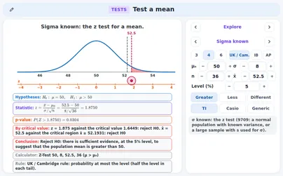
H0:μ=50, H1:μ>50, σ=8, n=36, xˉ=52.5: SE=8/6≈1.3333, z=2.5/(4/3)=1.875, p≈0.0304<0.05 (two-sided 0.0608>0.05). Reject H0 for the one-sided test.
Rule
The critical region for the sample mean
Rule 2 can be written for xˉ itself: reject H0 when xˉ is beyond c=μ0+zc⋅σ/n (for H1:μ>μ0), where zc is the normal critical value. Two-tailed: μ0±zcσ/n with zc for half the level. It gives the same decision as the p-value.
Example
Same test: c=50+1.64485⋅4/3≈52.1931. Region xˉ≥52.1931; 52.5 lies in it: reject H0. Two-tailed at 5%: 50±1.960⋅4/3, region xˉ≤47.3867 or xˉ≥52.6133.
Rule
When sigma is not known: the t test
Usually σ is not known and the sample standard deviation s takes its place. Then t = \dfrac{\bar x - \mu_0}{s / \sqrt n} follows a t distribution with df=n−1, with heavier tails than the normal curve. Use t, not z, for any sample size under IB and AP (Cambridge allows z for a large sample).
A common mistake is to put s into the z formula and read the normal tail. The t distribution has heavier tails, so the true tail is bigger and the z p-value is too small: it overstates the evidence and can reject a null hypothesis that should stay. The difference is largest for small samples.
Example
The sample of the t test above, but xˉ=103.7: t=3.7/1.7898≈2.0673, df=11. The t test gives two-sided p≈0.0631>0.05: do not reject. The wrong z test gives p≈0.0387<0.05 and would reject.
Rule
Matched pairs: one sample of differences
When each route or subject is measured twice, the columns are not independent. Subtract pair by pair in a stated order and test the differences as one sample: H0:μd=0, t=dˉ/(sd/n), df=n−1. The order of subtraction decides the sign of dˉ and the direction of H1.
Example
Delivery minutes on 8 routes, before minus after: 2, 1, -1, 4, 2, 2, 2, 3; dˉ=15/8=1.875, sd≈1.4577. H1:μd>0: t≈3.6380, df=7, p≈0.0042<0.05: reject H0.
Rule
Conditions for a test for a mean
Trust a test for a mean when the sample is random, n is at most 10% of the population, and xˉ is close to normal: a normal population, or n large (UK / Cambridge and AP: at least 30; IB: above 30), or a small sample with no strong skew and no outliers. IB also says the underlying distribution must be normal for the t test.
Example
Ten fill levels: 48, 49, 50, 50, 51, 51, 52, 53, 54, 75. With n=10 look at the data: 75 is far above the upper fence Q3+1.5⋅IQR=57.5. A strong outlier in a small sample: the t test is not justified until the value is checked.
Rule
Which test fits the question?
Ask four questions. Which parameter? A proportion (exact binomial or normal test), a mean or a correlation. One sample or pairs? Pairs become one sample of differences. Is σ known? Known: z; unknown: t with df=n−1. Which conditions? Randomisation, 10%, counts or normality. For a correlation: t=rn−2/1−r2, df=n−2.
Example
(1) “Do 70% of seeds germinate?” A proportion in a sample of 20: exact binomial test. (2) “Does the machine fill 500 ml?” A mean with σ=4 known: z test. (3) “Is the delivery time lower after the change?” Pairs, σ unknown: t test on the differences.
Rule
Simulate the claim
Without a formula, a test can be run on the computer: draw many samples from the model of H0 with a seeded random generator and count the share that are at least as extreme as the observed result. That share estimates the p-value (CCSS S-IC.A.2: would this result make me question the model?).
Example
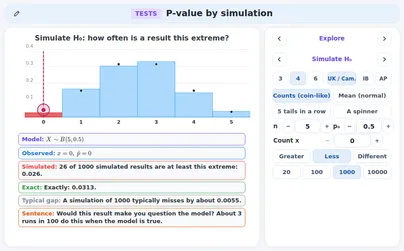
A coin model: tails with chance 1/2. Would 5 tails in a row make you doubt it? Exactly, (1/2)5=1/32=0.03125≈ 3.1%. Three presses of 100 simulated series in the application give 2,3,3 series with 5 tails: about 3 in 100, as expected.
Tip
A simulation next to the exact value
A simulated p-value is a share of R runs, so it carries its own error: it typically misses the exact value by about p(1−p)/R. To make the gap 10 times smaller you need 100 times as many runs. Put the exact value next to the simulated one whenever it is known.
Example
Exact 0.03125. Typical gap: R=100: 0.0174; 1000: 0.0055; 10000: 0.0017. The application’s first presses give 34 of 1000 (0.034) and 295 of 10 000 (0.0295): within one typical gap.
Rule
What the p-value says
Three sentences are always right. 1. The p-value is computed assuming H0 is true. 2. A small p-value says the result would be unusual if H0 were true. 3. A p-value that is not small is not evidence that H0 is true. Behind them: the p-value is the probability, assuming H0 is true, of a result at least as extreme as the observed one. It is about results, given H0, never about H0 itself.
Example
Seeds: p=0.0480. If H0 (70% germinate) is true, results at least as extreme as 10 of 20 happen about 4.8% of the time. That is below 5%, so the result would be unusual if H0 were true: reject H0 at the 5% level.
Rule
A large p-value is not evidence for H0
When the p-value is large, the sample is not unusual if H0 is true. The honest conclusion is “do not reject H0 (not enough evidence against it)”. It is not evidence for H0: other parameter values would fit the sample just as well, and a small sample cannot tell them apart.
Example
A fair coin is flipped 20 times and shows tails 8 times. H0:p=0.5, H1:p=0.5: the smaller tail P(X≤8)=0.2517, so the two-sided p-value is far above 0.05: do not reject H0. But p=0.4 gives exactly 20⋅0.4=8 tails on average, so the sample fits p=0.4 just as well.
Watch out!
Misreading 1 (WRONG): the probability that H0 is true
WRONG: “The p-value is the probability that H0 is true.” Verdict: the p-value is calculated assuming H0 is true, so it cannot also measure how likely H0 is. It is a probability of results given H0. A hypothesis about a population is either right or not; the p-value gives it no probability.
Example
Seeds: p=0.0480 does not say that the supplier is right with probability 0.0480. It says that if the supplier is right, results as extreme as 10 of 20 happen about 4.8% of the time.
Watch out!
Misreading 2 (WRONG): the probability of chance alone
WRONG: “The p-value is the probability that the result is due to chance alone.” Verdict: the p-value starts from the assumption that only chance is at work (H0) and asks how often results this extreme then occur. It does not split the result into a part due to chance and a part due to something else.
Example
A delivery check gives p=0.0480 for 10 late parcels of 20 against p0=0.3. That is not “a 4.8% chance that the result is a fluke”: it is the share of samples of 20 parcels, from a company whose late share really is 0.3, that give 10 or more late parcels.
Watch out!
Misreading 3 (WRONG): 1 − p as the chance of H1
WRONG: “1−p is the probability that the alternative hypothesis is true.” Verdict:1−p is the probability, assuming H0 is true, of a result that is less extreme than the observed one. It is still a statement under H0, and says nothing about how likely H1 is.
Example
Seeds: 1−p=1−0.0480=P(X≥11) under B(20,0.7), the area of the bars right of 10, about 0.952. It is not “a 95% chance that the seeds are worse than claimed”.
Watch out!
Misreading 4 (WRONG): a small p-value proves H1
WRONG: “A small p-value proves the alternative hypothesis.” Verdict: a small p-value is evidence against H0, with a known risk α of rejecting a true H0. Evidence is not proof: at the 5% level about 1 test in 20 of true null hypotheses is rejected. Say “reject H0: there is evidence that …”.
Example
Among 1000 tests of true null hypotheses at 5%, about 1000⋅0.05=50 reject, each with a small p-value, and none proves its alternative. In the seeds example (p=0.0480) the right sentence is that there is evidence that fewer than 70% germinate.
Watch out!
Misreading 5 (WRONG): a large p-value shows H0 is true
WRONG: “A large p-value shows that H0 is true.” Verdict: a large p-value only says that the sample is not unusual if H0 is true. Many other parameter values would also give such a sample. The right words: “do not reject H0: there is not enough evidence …”.
Example
Bottling: target 500 ml, σ=4, 16 bottles with mean 498.5: z=−1.5000, two-sided p=0.1336>0.05. Right: do not reject H0. It does not show that the mean is 500: a machine 1 ml low would give a similar sample.
Tip
Significant is not the same as important
A test says whether a difference can be told apart from sampling variation, not whether it matters. With a very large sample even a tiny difference gives a small p-value; with a small sample even a large one may not. Report the size of the difference next to the p-value, and look at an interval for it.
Example
H0:p=0.5 with p^=0.51. For n=10000: SE=0.0050, z=0.01/0.0050=2.0000, two-sided p≈0.0455: reject at 5%. For n=100: z=0.2000, p≈0.8415: nothing. The share is the same 51% both times.
Rule
The test for a correlation
Could a sample of n pairs give such an r when the population correlation ρ is 0? Test H0:ρ=0 with t = \dfrac{r \sqrt{n - 2}}{\sqrt{1 - r^2}}, \qquad df = n - 2, or compare ∣r∣ with the critical value of r from a table: the same decision. Conditions: random pairs, a roughly linear pattern.
Example
n=10, r=0.7, two-tailed 5%: t=0.78/0.51≈2.7724, df=8, p≈0.0242<0.05. Critical t=2.3060, so critical r=2.3060/2.30602+8≈0.6319<0.7: reject H0; there is evidence of a linear association.
Tip
The shuffle test beside it, and correlation is not cause
Shuffle the y values at random against the x values: this destroys any link, so each shuffle shows an r that “no association” gives. The share of shuffles with ∣r∣ at least the observed ∣r∣ estimates the p-value, close to the t test. Even a significant r shows an association, not that one variable causes the other.
Example
The application’s ten pairs (x=1,…,10; y=2,5,3,7,4,6,9,5,8,7): r≈0.694, t≈2.726, p≈0.0260. Of 1000 seeded shuffles 39 have ∣r∣≥0.694 (0.039; another press: 31). All 10! orderings give the exact 0.0307.
Definition
Type I and Type II errors
Type I error: reject H0 when H0 is true; probability α. Type II error: do not reject H0 when H0 is false; probability β. The power1−β is the probability of rejecting H0 when it is false. Which error costs more depends on the context, so say in words what each one means.
Example
Fire alarm, H0: “no fire”. Type I: it rings with no fire (a false alarm). Type II: there is a fire and it stays silent (a missed fire), the one to keep very small. Spam filter, H0: “not spam”. Type I: a good message goes to the spam folder. Type II: spam reaches the inbox.
Rule
Alpha, beta and power as areas
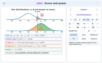
Draw the curve of xˉ under H0 (centre μ0) and under a true value μ1; the critical value c cuts both. α is the area of the H0 curve beyond c. β is the area of the μ1 curve before c. The power1−β is the area of the μ1 curve beyond c.
Example
H0:μ=50, σ=8, n=36, 5%, H1:μ>50: c=50+1.64485⋅4/3≈52.1931. True mean 53: z=(52.1931−53)/(4/3)≈−0.6051, β≈0.2725, power 0.7275: a mean of 53 is found about 73 times in 100.
Rule
The errors of a binomial test
For a binomial test the pictures are bar charts. Fix the critical region from H0 (say X≥c). Then α is P(X≥c) with p=p0, the actual level; β is P(X<c) with the true chance p1, and the power is P(X≥c) with p1. The same region cuts both bar charts.
Example
n=20, H0:p=0.3, region X≥10: α=P(X≥10)=0.0480. True chance p1=0.5: β=P(X≤9)=0.4119, power P(X≥10)=0.5881. With 20 trials the test misses a true p=0.5 in about 4 cases out of 10.
Rule
What changes the power
A bigger sample shrinks the standard error, so the curves overlap less. A truth farther from μ0 is easier to see. A larger level α gives more power but a larger Type I chance. A smaller σ works like a bigger sample. For a fixed sample a smaller α makes β larger; only more data lowers both errors.
Example
Previous test (power 0.7275 at 53): n=144: SE=0.6667, β≈0.0022, power 0.9978. Truth 55: β≈0.0176. Level 1%: β≈0.5304, power only 0.4696. σ=4 gives SE=0.6667, as n=144 does.
Tip
Everyday test 1: seed germination
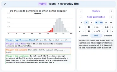
A binomial test in four stages. 1H0, H1 and the level. 2 The null distribution with the observed result. 3 The p-value, or the critical region and the actual level. 4 The conclusion in context, in the frame of your course, and the error that could have been made: a Type II error after “do not reject”, a Type I error after “reject”.
Example
80% germination claimed; 28 of 40 germinate. H0:p=0.8, H1:p<0.8, 5%: P(X≤28)=0.0875>0.05. Critical region X≤27 (actual level 0.0432); 28 is not in it. Do not reject H0. If the seeds really are worse, this is a Type II error.
Tip
Everyday test 2: a bottling machine
A mean with known σ: the z test, two-sided because the question is “is it off target?”. The critical region for xˉ is the target ±zcSE. Add the power: how often would the test notice a machine that is a given number of millilitres low? A test that notices only half of the real faults leaves a lot to the Type II error.
Example
Target 500 ml, σ=4, 16 bottles, mean 498.5: SE=1, z=−1.5000, two-sided p=0.1336>0.05. Region xˉ≤498.0400 or xˉ≥501.9600: 498.5 is inside the acceptance region, do not reject H0. If the machine is really 2 ml low, the power is only 0.5160.
Tip
Everyday test 3: delivery times
Before-and-after data on the same routes are matched pairs: test the differences with a t test. A confidence interval for the mean difference is a cross-check: if 0 lies outside the 95% interval, a two-sided test at 5% rejects H0:μd=0 as well; if 0 lies inside, it does not.
Example
Eight routes, before minus after 2, 1, -1, 4, 2, 2, 2, 3: dˉ=1.875, t≈3.6380, df=7. One-sided p≈0.0042: reject; two-sided 0.0083. The 95% interval (0.6563,3.0937) (t∗=2.3646) excludes 0, as the two-sided test does. If the change did nothing, rejecting would be a Type I error.
Tip
Everyday test 4: is a spinner fair?
A spinner has four equal sectors, so a fair one lands on a chosen sector with chance 1/4. A binomial test checks one sector. The question decides the tails: “comes up too often” is one-sided, “is the spinner fair?” is two-sided. The same data can pass one question and not the other, so choose the question before spinning.
Example
A sector comes up 9 times in 20 spins (5 expected). H0:p=0.25. One-sided: P(X≥9)=0.0409<0.05, reject; region X≥9, actual level 0.0409. Two-sided (AP): 2⋅0.0409=0.0819>0.05, do not reject. Both answer different questions.
Tip
Which course asks what
Cambridge 9709: P651 to P655 (terms, binomial test, mean of a normal population, Type I and II errors). UK A level (DfE, Edexcel 9MA0, AQA 7357): O1 to O3. IB AI: SL411 (hypotheses, levels, p-values, the t-test, one- and two-tailed) and AHL418 (critical values and regions, a mean, a binomial proportion, ρ = 0, errors). AP: 35 to 38, 44, 45. CCSS: S-ICA2. NL wiskunde D vwo: et-08. Not here: Poisson tests, chi-squared tests, two-sample tests; no MEB, GCSE / IGCSE, NL A or C.
Example
An IB AI pupil needs the cards on hypotheses, levels, the p-value, the t test, tails, critical regions, the one-tailed binomial test, the correlation test and the errors. A Cambridge 9709 pupil needs the binomial test with exact probabilities, the actual level, the z test and the errors. An AP pupil needs the conditions, the z test for a proportion, the t test and the AP wording.
Exercises
A cereal box says it holds 500 g on average. A buyer thinks the boxes hold less. State H0 and H1 and say whether the test is one-tailed or two-tailed. Easy
Show solution
The parameter is the population mean μ of the content of a box.
The equality goes in H0: H0:μ=500.
The buyer thinks “less”, so H1:μ<500. One direction only: one-tailed.
H0:μ=500, H1:μ<500; one-tailed
Check → the equality is in H0 only, and H1 names the direction of the buyer’s doubt.
Write H1 and say whether the test is one-tailed or two-tailed. (a) “Has the share of late parcels gone up from 0.3?” (b) “Is the spinner fair?” (a sector should come up with chance 0.25). Easy
Show solution
(a) “Gone up” names a direction: H0:p=0.3, H1:p>0.3, one-tailed.
(b) “Fair?” names no direction: H0:p=0.25, H1:p=0.25, two-tailed.
Check → the direction comes from the words of the question, not from the data.
A test gives the p-value 0.0304. Decide at the 5% level and at the 1% level whether to reject H0 (rule: reject if p≤α). Easy
Show solution
At 5%: 0.0304≤0.05, so reject H0.
At 1%: 0.0304>0.01, so do not reject H0.
Reject H0 at 5%; do not reject H0 at 1%
Check → the level is chosen before the test; the same p-value can pass one level and not the other.
H0:μ=120, H1:μ>120, σ=15 is known, n=25 and xˉ=124.5. Find z and the p-value (4 decimal places). Easy
Show solution
The standard error is SE=15/25=3.
Then z=(124.5−120)/3=4.5/3=1.5000.
The p-value is the upper tail: P(Z>1.5000)≈0.0668.
z=1.5000 and p≈0.0668
Check → 0.0668>0.05, so at the 5% level H0 is not rejected.
A fair coin is a model for 10 flips: X∼B(10,0.5). A series gives 9 tails. Find the exact p-value P(X≥9) as a fraction and as a decimal (4 decimal places). Easy
Show solution
Every outcome of 10 flips has probability (1/2)10=1/1024.
P(X=9)=10/1024 and P(X=10)=1/1024.
P(X≥9)=(10+1)/1024=11/1024≈0.0107.
11/1024≈0.0107
Check → 11/1024<0.05, so the result would be unusual for a fair coin: the model is doubted at the 5% level.
A two-tailed z test at the 5% level gives z=−2.3. Do you reject H0? Find the two-sided p-value (4 decimal places). Easy
Show solution
The critical values of a two-tailed test at 5% are ±1.960.
∣−2.3∣=2.3>1.960, so z lies in the critical region: reject H0.
One tail: P(Z<−2.3)=0.0107. Two-sided: 2⋅0.0107=0.0214, below 0.05.
Reject H0; two-sided p≈0.0214
Check → both rules agree: z in the critical region and p<0.05.
H0:p=0.2, H1:p>0.2 for n=15 trials, level 5%. Find the critical region and its actual significance level (4 decimal places). Medium
Show solution
Under H0, X∼B(15,0.2), with mean 15⋅0.2=3.
Search from the top: P(X≥7)=0.0181≤0.05 but P(X≥6)=0.0611>0.05.
So the critical region is X≥7 and the actual level is 0.0181, not 0.05.
X≥7; actual level 0.0181
Check → 0.0181≤0.05<0.0611: the region is the largest one that fits the level.
A poll of 100 pupils finds 62 who cycle to school. Test H0:p=0.5 against H1:p=0.5 with the normal test: find z and the two-sided p-value (4 decimal places) and write the AP conclusion at 5%. Medium
Show solution
SE=0.5⋅0.5/100=0.05 and z=(0.62−0.5)/0.05=2.4000.
One tail P(Z>2.4000)=0.0082; two-sided 2⋅0.0082=0.0164<0.05.
AP: Reject H0: there is convincing evidence that the true share of pupils who cycle is different from 0.5.
z=2.4000, p≈0.0164; reject H0
Check → the exact two-sided value is 0.0210, also below 0.05.
Nine bottles have mean volume 21.4 cl and s=3. Test H0:μ=20 against H1:μ=20 at 5%, σ unknown: find t, df, the two-sided p-value (4 decimal places) and decide. Medium
Show solution
SE=3/9=1 and t=(21.4−20)/1=1.4000, df=9−1=8.
Two-sided p=2⋅P(T8>1.4000)≈0.1991>0.05; also 1.4000<t∗=2.3060. Do not reject H0.
t=1.4000, df=8, p≈0.1991; do not reject H0
Check → the wrong z test would give the smaller p≈0.1615.
Five routes are timed before and after a change (minutes saved): 3, 4, 1, 5, 2. Test H0:μd=0 against H1:μd>0 at 5%: find t and the one-sided p-value (4 decimal places). Medium
Show solution
dˉ=15/5=3; squares of the deviations 0+1+4+4+1=10, so sd2=2.5 and sd≈1.5811.
t=3/(1.5811/5)≈4.2426 with df=4; one-sided p≈0.0066<0.05. Reject H0.
t≈4.2426, p≈0.0066; reject H0
Check → the critical value for df=4, one-tailed 5%, is 2.1318<4.2426.
A student tests H0:p=0.3 with n=20 and the rule “reject H0 if X≥9”. What is the probability of a Type I error (4 decimal places)? Is the rule within a 5% level? Medium
Show solution
A Type I error is rejecting a true H0. Under H0, X∼B(20,0.3).
Its probability is P(X≥9)=0.1133.
0.1133>0.05, so the rule is not within 5%. The rule X≥10 has 0.0480 and does fit.
0.1133; no, it is above 5%
Check → the probability of the region is the actual significance level: it must be at most the level.
H0:μ=100, H1:μ>100, σ=15, n=25, level 5%. Find the critical value c of xˉ and the probability β of a Type II error when the true mean is 106, and the power (4 decimal places). Medium
Show solution
SE=15/5=3 and c=100+1.64485⋅3≈104.9346.
β=P(xˉ<c) with mean 106: z=(104.9346−106)/3≈−0.3551, so β≈0.3612.
The power is 1−0.3612=0.6388.
c≈104.9346, β≈0.3612, power ≈0.6388
Check → 0.3612+0.6388=1: the power and β share the true-value curve.
A binomial test of H0:p=0.5 against H1:p=0.5 uses n=25 at 5% (UK / Cambridge rule). Find the critical region, the acceptance region and the actual level (4 decimal places). Hard
Show solution
Each tail at most 0.025; X∼B(25,0.5). P(X≤7)=0.0216≤0.025 but P(X≤8)=0.0539>0.025, so the lower part is X≤7.
By symmetry the upper part is X≥18; acceptance region 8≤X≤17. Actual level 2⋅0.0216=0.0433.
X≤7 or X≥18; acceptance 8≤X≤17; actual level 0.0433
Check → IB does not examine this two-tailed binomial test.
H0:p=1/2, H1:p>1/2, n=4, x=4, level 6.25%. Find the p-value and decide under UK / Cambridge, IB and AP. Hard
Show solution
P(X≥4)=(1/2)4=1/16=0.0625, exactly equal to the level 6.25%.
UK / Cambridge and AP: reject when p≤α, so reject. IB: reject only when p is strictly below the level, so do not reject.
p=1/16=0.0625; UK / Cambridge reject, IB do not reject, AP reject
Check → the conventions differ only for a p-value exactly on the level.
H0:p=0.3, H1:p>0.3, n=50, x=21. Find the normal p-value, the exact p-value and the p-value with the continuity correction (4 decimal places). Which normal value is closer to the exact one? Hard
Show solution
p^=0.42, SE=0.21/50=0.0648, z=0.12/0.0648=1.8516 and P(Z>1.8516)=0.0320.
Corrected: z=(20.5−15)/3.2404=1.6973 and P(Z>1.6973)=0.0448. Exact: P(X≥21)=0.0478. The corrected value is closer.
Normal 0.0320, corrected 0.0448, exact 0.0478; the corrected value is closer
Check → the counts are 15 and 35, both at least 10, so the approximation is allowed.
A machine should fill 12 cl with known σ=0.5 cl. A sample of 25 has mean 11.8 cl. Test H0:μ=12 against H1:μ=12 at 5%: find z, the two-sided p-value (4 decimal places), the critical region for xˉ and decide. Hard
Show solution
SE=0.5/5=0.1, z=(11.8−12)/0.1=−2 and the two-sided p=2⋅P(Z>2)=0.0455<0.05.
Critical region 12±1.960⋅0.1: xˉ≤11.8040 or xˉ≥12.1960. Since 11.8<11.8040, reject H0.
z=−2, p≈0.0455; reject H0
Check → a borderline result: say there is evidence, not proof, that the mean fill differs from 12 cl.
A sample of 16 has mean 47.2 and s=5.6. Test H0:μ=45 against H1:μ>45 with the t test: find t, df and the p-value (4 decimal places). Decide at 5% and at 10%. Hard
Show solution
SE=5.6/4=1.4, t=(47.2−45)/1.4=1.5714, df=16−1=15.
One-sided p=P(T15>1.5714)≈0.0685: above 0.05, do not reject at 5%; below 0.10, reject at 10%.
t=1.5714, df=15, p≈0.0685; do not reject at 5%, reject at 10%
Check → at 5% the critical value is 1.7531>1.5714; the wrong z test would give p≈0.0580.
The test of H0:p=0.3 against H1:p>0.3 with n=20 uses the region X≥10. Find β and the power when the true chance is p1=0.4 and when it is p1=0.6 (4 decimal places). Hard
Show solution
The region stays the same; only the distribution changes: β=P(X≤9) and power =P(X≥10) with p1.
p1=0.4: β=0.7553, power 0.2447. p1=0.6: β=0.1275, power 0.8725. A truth farther from 0.3 is found much more often.
p1=0.4: β=0.7553, power 0.2447; p1=0.6: β=0.1275, power 0.8725
Check → β and the power add up to 1 each time.
A sample of 12 pairs has r=0.53. Test H0:ρ=0 against H1:ρ=0 at 5%: find t, df, the two-sided p-value and the critical r (4 decimal places), and write the UK / Cambridge conclusion for “study time and a test mark”. Hard
Show solution
t=0.5310/0.7191=1.9764 with df=12−2=10; two-sided p≈0.0763>0.05. Critical t=2.2281, so critical r≈0.5760>0.53.
Do not reject H0: there is not enough evidence, at the 5% level, to suggest a linear association between study time and test mark.
t=1.9764, p≈0.0763, critical r=0.5760; do not reject H0
Check → ∣r∣=0.53 is below the critical r and p>0.05: the two rules agree.
Interactive applications for this topic
Free applications open with a free student account. Teachers can use all applications in a live lesson.