The population is the whole group we want to know about: every pupil of a school, every bag a machine fills. A number that describes the whole population is a parameter: the population mean μ, the standard deviation σ, the share p. A parameter is one fixed number, even when we do not know it.
Example
A chess club has 8 members, aged 12,14,14,15,16,16,17,20. The population is the 8 members.The parameters are μ=124/8=15.5 years and σ2=5; the share aged 16 or more is p=4/8=0.5.
Definition
Sample and statistic
A sample is the part of the population that we really look at. A number worked out from the sample is a statistic: the sample mean xˉ, the sample share p^, the sample standard deviation s. A statistic depends on which members were chosen.
Example
From the club we take 3 members, aged 14,16,20.Then xˉ=50/3≈16.67 and p^=32 (two of the three are 16 or older), while the parameters are μ=15.5 and p=0.5.
Rule
The estimate changes from sample to sample
A statistic used to guess a parameter gives an estimate: xˉ estimates μ, p^ estimates p. Another sample gives another estimate. So an estimate is near the parameter, but it is not the parameter: the parameter stays, the estimate changes.
Example
Three samples of 3 members: 14,16,20 and 12,14,15 and 15,16,17 give xˉ=16.67, 13.67 and 16, while μ=15.5 stays.The three estimates miss μ by +1.17, −1.83 and +0.5.
Definition
The sampling distribution
Take all possible samples of size n and work out the same statistic for each. These values form a distribution: the sampling distribution of the statistic. It tells how the statistic behaves from sample to sample; the cards that follow are about it.
Example
The population is the digits 0,1,2,3, each equally likely. All 16 samples of size 2 (with replacement) give xˉ=0,0.5,…,3 with counts 1,2,3,4,3,2,1 out of 16.Their mean is 1.5=μ and their variance is 0.625, half of the population variance 1.25.
Rule
A random sample
In a simple random sample every member of the population has the same chance, and so has every possible sample. Nothing in the method leans to one side: over many samples the sample means are centred on μ. A sample chosen by who is easy to reach, or who wants to answer, has no such guarantee.
Example
We choose 3 of the 8 club members by drawing names. There are (38)=56 possible samples, each with chance 1/56, and every member is in the sample with chance 3/8=0.375.
Rule
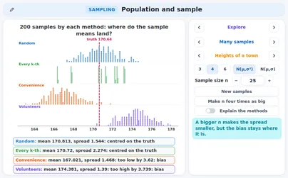
Four ways to choose a sample
Random: drawn by chance. Every k-th name of a list: fair as long as the list has no repeating pattern. Convenience (opportunity sampling): people who are easy to reach. Volunteers: people who choose to answer. The last two are biased: their sample means centre on the mean of the part of the population the method can reach.
Example
Samples of 2 from the club.All 28 pairs (random): the sample means average 15.5=μ. Only the 5 nearest members 12,14,14,15,16 (convenience): they average 14.2, that is −1.3 from μ. Only the 5 volunteers 15,16,16,17,20: they average 16.8, that is +1.3.
Watch out!
Bias and spread are two different things
A bigger sample makes the sample means gather closer together (less spread), but it does not move their centre. A big biased sample is still biased: it is only precisely wrong. Bias is about the centre, spread is about how far the estimates scatter.
Example
The 5 nearest members 12,14,14,15,16 (convenience), samples of 2 and of 4 without replacement.Both have the centre 14.2, which is −1.3 from μ=15.5. But the standard deviation of xˉ falls from 0.812 (n=2) to 0.332 (n=4).
Tip
Is the method poor? Three questions
To judge a sampling method ask three questions. Who can be chosen? Is anyone left out? Does everyone have the same chance?Who answers? Do those who answer differ from the rest? If one answer is no, say in which direction the result is pushed, and remember that a larger sample does not repair it.
Example
A shop asks the first 100 customers on Saturday morning whether the opening hours are good.Who can be chosen: only Saturday morning customers; evening and weekday customers are left out. The result is pushed towards people who like mornings, and asking 1000 of them would not repair that.
Rule
From a sample to an informal inference
We use an estimate to say something about the parameter, but only informally: "the share is probably around 0.28". The sampling distribution shows how far an estimate can be off. A sample does not give the exact value, and another random sample would give another statement: that is the limit of sampling.
Example
In a sample of 50 pupils, 14 say yes: p^=14/50=0.28.If the true share were 0.3, then a share 0.957 of all such samples has p^ between 0.17 and 0.43 (counts 9 to 21, exact binomial). So 0.28 is an ordinary result for p=0.3, but one sample cannot prove that p is exactly 0.3.
Definition
The sample mean is a random variable
Before the sample is drawn, the sample mean Xˉ=nX1+X2+⋯+Xn is a random variable: it takes different values for different samples. After the draw we have one value xˉ. The capital Xˉ is the variable, the small xˉ one observed value.
Example
A population table: x=0,1,2,3 with probabilities 0.1,0.4,0.3,0.2. Then μ=1.6 and σ2=0.84.One sample of 2 is (1,3): xˉ=2. Another is (0,2): xˉ=1. Different samples, different values of Xˉ.
Rule
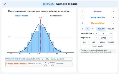
The expected value of the sample mean
The expected value of the sample mean is the population mean: E(Xˉ)=μ for every n. Over all samples the sample means balance at μ, so xˉ is an unbiased estimate of μ. This does not say that one sample mean equals μ.
Example
The table above with n=2: Xˉ takes the values 0,0.5,1,1.5,2,2.5,3 with probabilities 0.01,0.08,0.22,0.28,0.25,0.12,0.04.Then E(Xˉ)=∑xˉ⋅P(Xˉ=xˉ)=1.6=μ.
Rule
The variance and the standard error
The values in a random sample are independent, so their variances add: Var(X1+⋯+Xn)=nσ2. Dividing the sum by n divides the variance by n2: Var(Xˉ)=nσ2. The standard deviation of Xˉ is nσ; it is called the standard error.
Example
Test scores have σ=15. The mean of n=9 scores has Var(Xˉ)=225/9=25, so the standard error is 15/9=5.For the table above and n=2: 0.84/2=0.42, and that is what the exact table of Xˉ gives.
Rule
More values, a narrower mean
The standard error σ/n falls as n grows, but only like 1/n: four times as many values halve it. It is the spread of Xˉ that falls; the spread σ of the population stays as it is.
Example
With σ=15 and n=1,4,16 the standard error is 15, 7.5 and 3.75: each curve is twice as narrow as the one before.The mean of 16 values scatters four times less than one value.
Rule
The exact table of the sample mean
For a small population table the whole distribution of Xˉ can be listed: write down every sample, work out its xˉ and add the probabilities of equal values. Then every probability about Xˉ is a sum of table entries, with no approximation.
Example
Same table, n=2 (picture): P(Xˉ≤1)=0.01+0.08+0.22=0.31.For n=5 the same method gives E(Xˉ)=58, Var(Xˉ)=12521=0.168 and P(Xˉ≤1)=2500277=0.1108.
Rule
A normal population gives a normal sample mean
If the population is normal, X∼N(μ,σ2), then Xˉ∼N(μ,σ2/n) exactly, for every n: a sum of independent normal variables is normal. So P(Xˉ<c) is a normal probability whose standard deviation is σ/n.
Example
Test scores X∼N(100,152). One score: P(X>110)=P(Z>10/15)≈0.2525.The mean of n=9 scores: Xˉ∼N(100,52) and P(Xˉ>110)=P(Z>2)≈0.0228. A mean of 9 is far less likely to be this high.
Rule
A probability about the sample mean
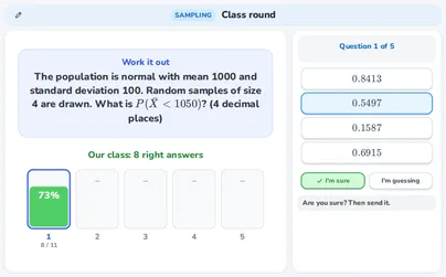
To find P(Xˉ<c): (1) state the model, Xˉ∼N(μ,σ2/n); (2) standardise with the standard error, z=σ/nc−μ; (3) read Φ(z) from the table, or type the calculator line with σ/n in the place of the standard deviation.
Example
Reaction times are N(250,402) ms and n=16: σ/n=40/4=10.P(Xˉ<235): z=(235−250)/10=−1.5, so the probability is Φ(−1.5)≈0.0668. Calculator: \texttt{normalcdf(-1E99, 235, 250, 10)}. One reaction below 235 has ≈0.3538.
Watch out!
σ or σ / √n?
A common mistake: standardising a sample mean with σ instead of σ/n. Ask: is the question about one value, or about a mean of n values? One value: σ. A mean of n values: σ/n.
Example
Heights N(170,82), the mean of n=4 pupils, P(Xˉ>174).Right: z=4/(8/2)=1, probability ≈0.1587. Wrong: z=4/8=0.5 gives 0.3085, which is the probability for one pupil taller than 174 cm.
Rule
The conditions
Before using the normal model for Xˉ check three conditions. Random: the sample is a random sample. 10%: when sampling without replacement, n is at most 10% of the population size N, so the draws are almost independent. Normal: the population is normal, or n is large (central limit theorem); a small n with strong skew or outliers fails.
Example
A school has N=300 pupils.A random sample of n=25 passes the 10% condition (300/10=30≥25). A sample of n=40 does not (40>30): the draws are no longer nearly independent.
Definition
The sample proportion
The sample proportion is p^=nX, where X is the number in the sample with the property. For a random sample that is small against the population, X∼B(n,p) with p the share in the population. So p^ is a random variable and an unbiased estimate of p: E(p^)=p.
Example
A poll of n=50 pupils: 14 say yes, so p^=14/50=0.28.Another sample of 50 may give 17 yes: p^=17/50=0.34. The share p in the school stays the same; only the sample changes.
Rule
The mean and the standard deviation of p̂
E(p^)=p and Var(p^)=np(1−p), so SD(p^)=np(1−p). This follows from p^=X/n with E(X)=np and Var(X)=np(1−p). As for the mean, four times as many people halve the standard deviation.
Example
p=0.3 and n=50: Var(p^)=0.3⋅0.7/50=0.0042 and SD(p^)=0.0042≈0.0648.With n=200 (four times as many) it is ≈0.0324, half of it.
Rule
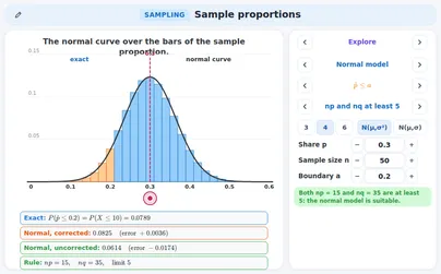
The exact distribution of p̂
The exact distribution of p^ is the binomial distribution with the counts divided by n: P(p^=k/n)=P(X=k). An event about p^ is an event about the count: p^≤0.2 means X≤0.2n. No approximation is needed.
Example
p=0.3 and n=50: p^≤0.2 is X≤10, so P(p^≤0.2)=P(X≤10)≈0.0789.Calculator: \texttt{binomcdf(50, 0.3, 10)}.
Rule
The normal model and the continuity correction
For large n the bars of p^ follow the normal curve N(p,p(1−p)/n). The bars are discrete: treat p^≤a as the count X≤k and use the continuity correction with the boundary k+21. The corrected value is usually much closer to the exact one than the uncorrected value.
Example
The same example: X≈N(15,10.5).Corrected: z=(10.5−15)/10.5≈−1.39, so Φ(−1.39)≈0.0825. Uncorrected: z=(10−15)/10.5≈−1.54, so 0.0614. The exact value is 0.0789: errors 0.0036 and 0.0174.
Rule
The conditions for p̂
The normal model for p^ needs a random sample, n at most 10% of the population, and enough successes and failures: np and nq=n(1−p) both at least 10 (the AP rule) or at least 5 (the Cambridge rule). Otherwise the bars are lopsided and a normal curve does not follow them.
Example
n=50, p=0.3: np=15 and nq=35, both at least 10: fine.n=20, p=0.1: np=2 is too small. The bar p^=0 has 0.920≈0.1216 and sits against the edge, and the curve ignores that p^ cannot be negative.
Rule
Say it as a sentence about samples
Say a probability about p^ (or Xˉ) as a sentence about samples: "In random samples of size n from a population in which …, the chance that … is about …". The probability belongs to the statistic. The parameter appears in the condition of the sentence, not in the event.
Example
In random samples of 50 from a population in which 30% support the plan, the chance that at most 20% of the sample support the plan is about 0.0789.
Watch out!
A probability about the sample, not about p
A common mistake: to read the 0.0789 as a statement about the parameter, as if p were the thing that varies. The share p in the population is one fixed number; it is the samples that vary. The sentence is about the sample share p^ in the samples drawn from this population. The same holds for a mean: a statement about Xˉ belongs to the samples, not to μ.
Example
Better: "If the share is 30%, then about 7.9% of the samples of 50 have at most 20% supporters." Here 30% is given, and the 7.9% counts samples.A poll that finds 20% does not turn the share into 20%; it is one sample from the many that could have been drawn.
Rule
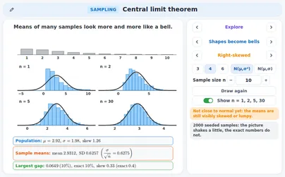
Shapes become bells
The central limit theorem: whatever the shape of a population (with a mean and a standard deviation), the distribution of Xˉ comes closer to the normal curve N(μ,σ2/n) as n grows. The bars of Xˉ turn into a bell that keeps the centre μ and gets narrower.
Example
A right-skewed population (the values 1 to 10, mean 2.925, σ≈1.984). The pictures show the exact distribution of Xˉ for n=1,2,5,30 with the normal curve: lopsided for n=1, a bell for n=30.The skew of Xˉ is the skew of one value divided by n: 1.26, 0.89, 0.56 and 0.23.
Rule
How large is large?
How large n must be depends on the population. The rules: Cambridge says "a large sample" without a number, IB says that n>30 is considered sufficient in examinations, AP uses n≥30. They are rules of thumb. The application also measures the biggest gap between a bar of Xˉ and the curve as a share of the peak, and the skew of Xˉ; it calls them close to normal when the gap is under 8% and the skew under 0.2.
Example
Right-skewed population, gap (share of the peak) and skew of Xˉ:n=5: 14.9% and 0.56; n=10: 10.1% and 0.40; n=30: 5.3% and 0.23; n=100: 3.0% and 0.13.At n=30 the gap is small but the skew 0.23 is still above 0.2; at n=100 both are small. A normal-like population is close to normal from n=1 (gap 4.4%).
Watch out!
A very skewed population
Caution (AP): when the population is extremely skewed, or holds one huge value, n=30 may not be enough. Look at the picture of Xˉ, not only at the number n.
Example
A population where 99% of the values are 1 and 1% are 10 (mean 1.09).A sample of 30 holds no 10 with chance 0.9930≈0.7397, so in about 74% of the samples xˉ=1 exactly; in the others it jumps in steps. The skew of Xˉ is still 1.80 at n=30 and 0.98 at n=100 (gap 15% and 31% of the peak).
Rule
Sums and means
The sum S=X1+⋯+Xn and the mean Xˉ=S/n are the same draws on two scales. When Xˉ is close to normal, so is S: S≈N(nμ,nσ2) and Xˉ≈N(μ,σ2/n). The sum has mean nμ and standard deviation σn.
Example
The right-skewed population, n=30: S has mean 30μ=87.74 and variance 30σ2=118.13, so standard deviation 10.869.P(S≥100): exact 0.1410; normal with the continuity correction (boundary 99.5, z=1.08) 0.1395; without (z=1.13) 0.1296. The event Xˉ≥100/30 is the same event.
Watch out!
The theorem is about the sample mean
A common mistake: "with a large sample the data become normal". The histogram of one large sample keeps the shape of the population. The theorem is about the distribution of Xˉ over many samples. A larger sample does not change the population; only the distribution of Xˉ narrows and rounds off.
Example
The right-skewed population has skew 1.26, so a histogram of 30 values taken from it is lopsided too.The means of many samples of 30 have skew 1.26/30≈0.23: they are the ones that look like a bell.
Definition
Estimator and unbiased
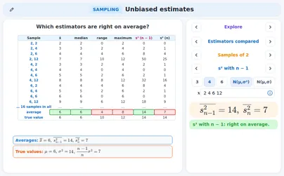
An estimator is a rule that turns a sample into an estimate of a parameter (xˉ for μ). It is unbiased if its expected value is the parameter: averaged over all samples the estimates hit the parameter. A biased estimator is wrong on average, always on the same side.
Example
The population is 2,4,6,12: μ=24/4=6 and σ2=56/4=14.We take all 16 samples of size 2 (with replacement) and average an estimator over them. It is unbiased when that average equals μ (or σ2), whatever the single samples do.
Rule
The sample mean is unbiased
The sample mean is an unbiased estimate of μ: E(Xˉ)=μ. You can check it by listing all the samples of a small population: the average of all the sample means is exactly μ.
Example
All 16 samples of size 2 from 2,4,6,12 (picture: the cell is xˉ of the row value and the column value). The 16 means add up to 96, so their average is 96/16=6=μ.Single means run from 2 to 12, the average is exactly right.
Rule
The sample variance with divisor n − 1
The sample variance s2=n−1∑(x−xˉ)2 (divisor n−1) is an unbiased estimate of σ2. With the divisor n it is too low on average: E(n1∑(x−xˉ)2)=nn−1σ2.
Example
The same 16 samples, σ2=14. Divisor n−1=1: the cells run from 0 to 50, add up to 224 and average 224/16=14=σ2.Divisor n=2 halves every cell: total 112, average 7=21⋅14.
Tip
Why n − 1?
The deviations from xˉ are smaller than the deviations from μ, because xˉ is the centre of this very sample. Exactly: ∑(x−μ)2=∑(x−xˉ)2+n(xˉ−μ)2. So ∑(x−xˉ)2 is too small by n(xˉ−μ)2, which is σ2 on average. Dividing by n−1 instead of n repairs that.
Example
The sample 2,12 from the population with μ=6: ∑(x−μ)2=16+36=52.With xˉ=7: ∑(x−xˉ)2=25+25=50 and n(xˉ−μ)2=2⋅1=2, and 50+2=52.
Rule
Computing x̄, s² and s
From data: xˉ=n∑x, s2=n−1∑(x−xˉ)2 and s=s2. From the sums n, ∑x and ∑x2: s2=n−11(∑x2−n(∑x)2). Keep fractions or many decimals until the end.
Example
n=10, ∑x=52, ∑x2=312: xˉ=526=5.2.∑x2−(∑x)2/n=312−270.4=41.6, so s2=41.6/9=45208≈4.6222 and s≈2.1499. With the divisor n: 41.6/10=4.16.
Tip
Sx and σx on the calculator
A calculator gives two standard deviations. Sx has the divisor n−1: the estimate of σ from a sample. σx has the divisor n: for a list that is the whole population. For a sample use Sx. Some makes and books write sn−1 and sn, or s and σ.
Example
Data 4;7;7;8;9: xˉ=7 and ∑(x−xˉ)2=9+0+0+1+4=14.Sx=14/4=3.5≈1.8708 and σx=14/5=2.8≈1.6733.
Watch out!
The maximum and the range are biased
Not every natural statistic is unbiased. The sample maximum is too low as an estimate of the population maximum, and the sample range too low as an estimate of the population range, because a sample usually misses the extremes. Their average over all samples lies below the target.
Example
2,4,6,12 and the 16 samples of size 2: the maximum averages 128/16=8 but the population maximum is 12; the range averages 64/16=4 but the population range is 12−2=10.
Watch out!
Unbiased is about the long run
Unbiased does not mean that one estimate is right: it means that the estimates are right on average over many samples. An unbiased estimator can still be far off in one sample. Also s is a slightly biased estimate of σ, even though s2 is unbiased for σ2.
Example
A seeded run (picture): population N(0,22), samples of 5. The running means of s2 settle near the targets: with divisor n−1 at 4 (green) and with divisor n at 54⋅4=3.2 (blue).For 2,4,6,12 the average of s over the 16 samples is 2.828, below σ≈3.742.
Rule
Unbiased and a small spread
Two unbiased estimators can differ in spread. The one with the smaller variance is better, because its single estimates lie closer to the target. A good estimator is unbiased (the centre is right) and has a small variance (little scatter).
Example
To estimate μ=6 from 2 draws: the first draw alone is unbiased with variance 14; xˉ is unbiased with variance 14/2=7.In the picture the 16 first draws (blue) are spread over 2 to 12, the 16 means (green) are less spread.
Rule
Poll size
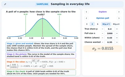
In a poll of n people the sample share has standard deviation p(1−p)/n, largest at p=0.5. About 95% of the polls land within 1.96 standard deviations of p. The margin shrinks like 1/n, so halving the margin needs four times as many people.
Example
With p=0.5 and n=100,400,1600 the standard deviation is 0.05, 0.025 and 0.0125.For a margin of 0.03: n≥1.962⋅0.25/0.032≈1067.1, so n=1068. (The exact binomial gives 0.953 for lying within 0.03.)
Rule
Bags of flour
A machine fills bags with mean weight μ and standard deviation σ. One bag varies with σ; the mean of n bags varies with σ/n. So a question about one bag below the label uses σ and a question about the mean of n bags uses σ/n.
Example
μ=1012 g, σ=15 g, label 1000 g, normal weights. One bag is under the label with chance Φ(−0.8)≈0.2119.The mean of n=9 bags: σ/9=5, z=−2.4, P(Xˉ<1000)≈0.0082.
Rule
Journey times
Journey times are usually skewed to the right: a few very long ones. The mean of n journeys is then only approximately normal, and better the larger n is. For a safe statement compare with the exact distribution, or look at the skew of Xˉ.
Example
Times 10,14,…,46 minutes with the right-skewed shape: mean 17.7 min, standard deviation 7.9 min, skew 1.26.n=10: P(Xˉ>22) is exactly 0.0467, the normal model says 0.0433 (skew of Xˉ0.40). n=30: exact 0.0027, normal 0.0015: the normal model underestimates the upper tail.
Rule
Lab readings
Repeat a measurement n times: the readings have a spread s, and the mean of the readings has the standard errors/n. The mean is more reliable than one reading, and four times as many readings halve the standard error.
Example
Readings 12.1,11.8,12.4,12.0,12.2,11.9: xˉ=72.4/6≈12.067, s≈0.2160, standard error s/6≈0.0882.With 24 readings of the same spread the standard error is 0.0441, half of it.
Tip
Which course asks what
Cambridge 9709 (Paper 6): sample and population, the sample mean as a random variable, the central limit theorem, unbiased estimates of the mean and variance. UK GCSE and A level: infer from a sample, population and sample, sampling techniques. IB (AA and AI): sampling and bias; AI HL: unbiased estimates and the central limit theorem. AP Statistics: sampling distributions of p^ and xˉ, conditions, unbiased estimators. Common Core: statistics as inference from a random sample. Netherlands: wiskunde A vwo, a statement about a population from a sample.
Example
A typical exam question: a population has mean 50 and standard deviation 8; a random sample of n=64.The standard error is 8/64=1, and P(Xˉ>51.5): z=1.5, so 1−0.9332=0.0668 (the central limit theorem, because n is large).
Exercises
A school has 800 pupils; 40 of them are asked how they travel and 22 say they cycle. Name the population and the sample. Is 22/40 a parameter or a statistic? Easy
Show solution
The population is all 800 pupils; the sample is the 40 who were asked.
22/40 is worked out from the sample, so it is a statistic: p^=22/40=0.55.
The share of all 800 who cycle is the parameter p; p^ estimates it.
Population: the 800 pupils; sample: the 40; p^=0.55 is a statistic
Check → another sample of 40 would probably give another p^; p would stay.
A random sample of 5 pupils has heights 63,71,66,68,62 cm. The mean height of all the pupils is μ=65 cm. Find xˉ and the difference xˉ−μ. Easy
Show solution
Add the heights: 63+71+66+68+62=330.
Divide by n=5: xˉ=330/5=66.
The difference is 66−65=+1 cm: this sample is a little above μ.
xˉ=66 cm, difference +1 cm
Check → the mean 66 lies between the smallest (62) and the largest (71) value.
A population has standard deviation σ=12. Find the standard error of the sample mean for n=36, and for a sample four times as large. Easy
Show solution
The standard error is σ/n=12/36=12/6=2.
Four times as large is n=144: 12/144=12/12=1.
Four times the sample size halves the standard error; the population spread σ=12 does not change.
2 for n=36 and 1 for n=144
Check → 144=4⋅36 and 1=2/2.
In a population 40% have a property. A random sample of n=100 is taken. Find the mean and the standard deviation of the sample share p^. Easy
Show solution
The mean of p^ is p=0.4.
The variance is p(1−p)/n=0.4⋅0.6/100=0.0024.
The standard deviation is 0.0024≈0.0490.
Mean 0.4, standard deviation ≈0.0490
Check → 0.0492≈0.0024.
A sample is 3,5,10. Find the sample mean xˉ, the sample variance s2 (divisor n−1) and s. Easy
Show solution
xˉ=(3+5+10)/3=18/3=6.
The squared differences: (3−6)2+(5−6)2+(10−6)2=9+1+16=26.
s2=26/(3−1)=13 and s=13≈3.606.
xˉ=6, s2=13, s≈3.606
Check → with divisor n you would get 26/3=326≈8.667, a smaller number than 13.
A school has 250 pupils. A random sample is taken without replacement and the 10% condition must hold. What is the largest sample size n? Easy
Show solution
The 10% condition says n≤10%⋅N.
Here N=250, so n≤250/10=25.
The largest sample has n=25 pupils.
n=25
Check → 25 is exactly a tenth of 250.
Scores are normal, N(500,402). Find P(Xˉ>510) for a random sample of n=16, and compare it with P(X>510) for one score. Medium
Show solution
The model is Xˉ∼N(500,102), because 40/16=10.
z=(510−500)/10=1, so P(Xˉ>510)=1−Φ(1)≈0.1587.
For one score z=10/40=0.25 and P(X>510)≈0.4013.
P(Xˉ>510)≈0.1587 against P(X>510)≈0.4013
Check → a mean of 16 scores is less likely to be far from 500 than one score, so 0.1587<0.4013.
A population has standard deviation σ=20. How large must a random sample be for the standard error of the mean to be at most 2.5? Medium
Show solution
We need 20/n≤2.5, so n≥20/2.5=8.
Square: n≥82=64.
n≥64
Check → 20/64=20/8=2.5.
In a population 60% agree; a random sample has n=80. Check the conditions and find P(p^<0.5) with the continuity correction (exact value 0.0271). Medium
Show solution
np=48 and nq=32, both at least 10: the normal model is fine.
p^<0.5 means X≤39, and X≈N(48,19.2).
Boundary 39.5: z=(39.5−48)/19.2≈−1.94, so P≈0.0262.
P(p^<0.5)≈0.0262 (exact 0.0271)
Check → without the correction (boundary 39) you get 0.0200, further from 0.0271.
A town has N=400 people. A random sample of n=60 is taken without replacement and asked a yes / no question; about 5% are expected to say yes. May the normal model for p^ be used? Medium
Show solution
Randomisation: the sample is random, so this condition is met.
10% condition: 10%⋅400=40 and 60>40: not met.
Counts: np=60⋅0.05=3, under 10 (and under 5): not met.
No: two conditions fail (10% and np), only the random one holds
Check → a sample of 40 or fewer would pass the 10% condition, but np would still be too small.
From a sample, n=8, ∑x=72 and ∑x2=702. Find xˉ and s2 with the divisor n−1, and compare with the divisor n. Medium
Show solution
xˉ=72/8=9 and 702−722/8=702−648=54.
s2=54/7=754≈7.7143; with the divisor n: 54/8=6.75.
xˉ=9, s2=54/7≈7.7143 (divisor n: 6.75)
Check → the divisor n gives the smaller number: 6.75<7.7143.
Population 1,3,8, all 9 samples of 2 with replacement. Show: xˉ averages μ, s2 (divisor n−1) averages σ2, divisor n gives half. Medium
Show solution
μ=4, σ2=26/3. The nine means add up to 36: average 4=μ.
The nine values of s2 add up to 78: average 78/9=326=σ2.
Divisor n=2 halves every value: average 313.
Averages: 4=μ and 26/3=σ2; with the divisor n: 13/3
Check → half of 26/3 is 13/3.
Journey times (right-skewed): mean 17.7 min, standard deviation 7.9 min, n=40. Find P(Xˉ>20) and name the rule that allows the normal model. Hard
Show solution
Central limit theorem: n=40≥30 (the AP rule). 7.9/40≈1.255.
z=(20−17.7)/1.255≈1.83, so P(Xˉ>20)≈0.0333.
The exact distribution of this skewed shape gives 0.0358: a little more.
P(Xˉ>20)≈0.0333 (exact: 0.0358)
Check → model and exact value differ by less than 0.003.
A poll wants a margin of 0.04, where the margin is 1.96 standard deviations of p^ (about 95%). Take the worst case p=0.5. How many people are needed? How many for a margin of 0.02? Hard
Show solution
1.960.25/n≤0.04, so n≥1.962⋅0.25/0.042=600.25: round up to n=601.
A margin of 0.02 is half, so four times as many: 1.962⋅0.25/0.022=2400.99, so n=2401.
n=601 for 0.04 and n=2401 for 0.02
Check → 2401 is about four times 601 (4⋅600.25=2401).
Bags of flour are normal, mean 1012 g, standard deviation 15 g. Find the chance that the mean of 9 bags is within 3 g of 1012 g, and the same for one bag. Hard
Show solution
Mean of 9: σ/9=5, so ∣z∣<3/5=0.6 and P=Φ(0.6)−Φ(−0.6)≈0.4515.
One bag: ∣z∣<3/15=0.2, so P≈0.1585.
About 0.4515 for the mean of 9 and 0.1585 for one bag
Check → the mean stays near 1012 more often than one bag: 0.4515>0.1585.
Samples of 50 from a population where 30% support a plan: P(p^≤0.2)≈0.0789. Which sentence is correct?A: As 0.0789 is small, the share is below 20%.B: If the share is 30%, 7.9% of samples have at most 20% supporters.C: This poll is wrong with chance 7.9%.Hard
Show solution
0.0789 counts samples for a given share, 30%. A and C turn it into a statement about the share or about “wrong”.
Only B keeps the share in the condition.
B
Check → B begins with “If the share is 30%”.
X1 and X2 are independent, with mean μ and variance σ2. Show that T1=(X1+X2)/2 and T2=(X1+2X2)/3 are both unbiased for μ and find which has the smaller variance. Hard
Show solution
E(T1)=(μ+μ)/2=μ and E(T2)=(μ+2μ)/3=μ: both are unbiased.
Var(T1)=(σ2+σ2)/4=21σ2.
Var(T2)=(σ2+4σ2)/9=95σ2>21σ2.
Both are unbiased; T1=Xˉ has the smaller variance
Check → 91+94=95; in the picture the row of T2 is wider.
A pupil computes the variance of samples of size 5 with the divisor n. The population variance is σ2=20. By what factor, and to what value, is the average of her results wrong? How does she repair it? Hard
Show solution
With the divisor n the average is nn−1σ2=54⋅20=16: too low by the factor 0.8.
She repairs it by dividing the same sum of squares by n−1=4 instead of n=5: 16⋅45=20.
Too low by the factor 0.8: 16 instead of 20; divide by n−1
Check → 16⋅5/4=20.
A convenience sample of 10000 has a mean that is typically 2 g too low. A random sample of 100 comes from a population with σ=15 g. Compare the standard errors and the kind of error. Hard
Show solution
The standard error for n=10000 is 15/100=0.15 g; for n=100 it is 15/10=1.5 g.
The big sample is precise but biased by about 2 g; more people would not change that. The random sample is unbiased: its error is only random.
The big sample has the smaller standard error (0.15 g against 1.5 g) but a bias of about 2 g; the random sample is unbiased
Check → bias is about the centre, and a larger n does not move it.
Interactive applications for this topic
Free applications open with a free student account. Teachers can use all applications in a live lesson.