İnteraktif Dersler

Statistics with a computer: big data sets

Lecture notes

Definition

Sort and filter a big data set

A big data set is a table of hundreds or thousands of rows: one row for each case and one column for each property. You cannot read it row by row, so you let the computer help. Sorting puts the rows in the order of one column, smallest or largest first; rows with the same value keep their order. A filter keeps only the rows that fit a rule. After a filter always say how many rows are left of all rows. In Sort and filter you choose the column, the direction and the filter and see the first rows, the counts and a summary of the column.
Example
The orders of a web shop: 1 000 rows. Sorted by delivery time, largest first, the first row is order 40 with 99 days (red: impossible). The filter Region is North keeps 354 of the 1 000 rows and removes 646 rows → . As a percentage → , so 35.4% of the rows are left.
#ValueItemsDelivery ▼Region4051.5399West33218.2199North51110.3199East654133699East75534.2299North
Watch out!

Impossible values

In real data some values cannot be right: a delivery of 99 days, a trip of 0 minutes, 24 hours of screen time in one day. They are often an error code or a slip. Look for them before you calculate: sort the column and look at both ends. They pull the mean and stretch a histogram. Leave them out with the filter Only plausible rows and work out the mean again. The median hardly moves, because it only looks at the middle.
Example
Delivery time: 7 of the 1 000 rows say 99 days. With them the mean is 4.786 days, so the total is . Without them → and rows are left, so the mean is days. The median stays 4.
Definition

The group summary

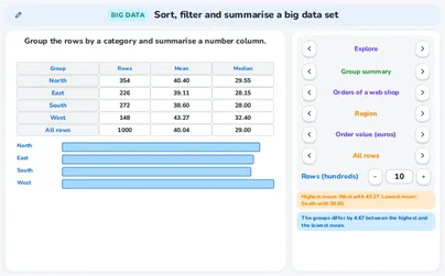
A group summary takes one category column (the rider) and one number column (the trip time) and gives, for every group, the number of rows, the mean and the median; the last row is for all rows. Compare the means of the groups and look at the medians too: a mean far above its median points to a few very large values. In Group summary you choose the category, the number column and whether impossible rows count.
Example
Trips with shared bikes (988 plausible trips): members 572 trips, mean 12.08, median 10 minutes; visitors 416 trips, mean 10.39, median 9. The members ride minutes longer on average. The mean of all trips is a weighted mean → and .
GroupRowsMeanMedianmember57212.0810visitor41610.399all rows98811.3710
Rule

The cross table: counts and percentages

A cross table counts the rows for every pair of two categories: one category gives the rows, the other the columns, and the totals stand at the edges. A percentage of each row says how every row is divided; use it to compare rows with each other. A percentage of each column says how every column is divided. Always say of which total you take the percentage. In Two categories you can switch between counts and both kinds of percentages.
Example
Region and type of customer (1 000 orders). The row West has 84 new and 64 returning customers → . As a percentage of the row → , so 56.8% of the orders from West are from new customers. As a percentage of the column → , so 14.5% of all new customers are in the West.
RegionnewreturningTotalNorth204150354East13987226South151121272West8464148Total5784221000
Rule

The histogram: class width and shape

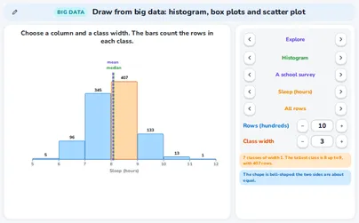
A histogram counts the rows in classes of equal width. The height of a bar is a number of rows, not a value. A value on the border of two classes goes into the class to its right. The class width matters: too narrow and the picture is ragged, too wide and the shape is hidden. Read the shape: bell-shaped, skewed to the right or to the left (a long tail on that side) or two peaks (two groups). The mean is pulled towards the long tail, so for a skewed-to-the-right shape the mean is above the median. In Histogram you choose the column and the class width.
Example
Delivery time without the impossible rows (993 rows), classes of width 1 day. The tallest class is 3 up to 4 with 260 rows. The tail runs to the right, to 14 days: the shape is skewed to the right, and the mean 4.12 is above the median 4.
12226025819597331573212468101214medianmeanDelivery time (days)
Rule

Box plots and outliers

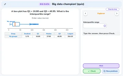
A box plot shows five numbers of a column: the smallest value, the lower quartile Q₁, the median, the upper quartile Q₃ and the largest value. The box holds the middle half of the rows and its length is the interquartile range IQR = Q₃ − Q₁. A value is an outlier when it lies more than 1.5 × IQR beyond the box: above Q₃ + 1.5 × IQR or below Q₁ − 1.5 × IQR. The whisker stops at the last value inside these fences. One box for each group lets you compare the medians, the spread and the outliers. In Box plots you choose a column and all rows or groups.
Example
Trip time of the visitors (416 trips): Q₁ = 6, median 9, Q₃ = 13, so IQR = . The upper fence is minutes: the whisker ends at 23 and 14 trips are outliers. For the members Q₁ = 7, Q₃ = 15, IQR = 8 and the fence is .
membervisitor01020304050607080Trip time (minutes)
Rule

The scatter plot, r and the line

A scatter plot puts two number columns against each other: one point for each row. With thousands of rows the application draws at most 500 points; the numbers use all rows. The correlation coefficient r lies between −1 and 1: the sign is the direction and the size is the strength (under 0.2 hardly any relation, 0.2 to 0.5 weak, 0.5 to 0.8 moderate, 0.8 and more strong). The regression line y = ax + b shows the trend, not a rule for every row. A relation in the data does not show that one column causes the other. In Scatter plot you choose the two columns.
Example
Trips: the distance against the battery used. For the 40 trips of the picture r = 0.90 (for all 988 trips r = 0.96), a strong relation going up, and the line is .86x + 0.94. At the line gives per cent.
0123456705101520r = 0.90Distance (km)Battery used (%)
Definition

Samples: random and biased

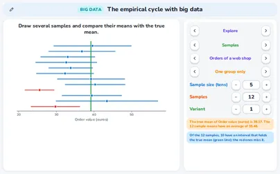
A sample is a part of the rows. In a random sample every row has the same chance to be chosen, so the sample means land on both sides of the true mean. A sample of one group only, or of volunteers (rows with large values join more easily), is biased: its means lie on one side of the true mean. A larger sample gives a smaller margin but does not repair bias. In Samples you draw several samples and see their means as dots with the true mean as a green line.
Example
Electricity use of 1 970 households: the true mean is 208.2 kWh a month. Eight random samples of 40 rows: 4 means are below and 4 above the true mean (the blue dots). Eight samples of volunteers: all 8 means are above it, from 222.6 to 262.0 (the orange dots): the sample is biased.
200225250275300Electricity (kWh a month)
Rule

The margin of a sample mean

The mean of a sample is not exactly the mean of all rows. The margin tells how far it can be off: margin = , with the standard deviation of the sample and its number of rows. The interval mean ± margin then holds the true mean for about 95 of 100 random samples. A larger n gives a smaller margin: for a margin half as big you need four times as many rows. Two groups differ for sure only when their intervals do not overlap.
Example
Trip time. For the members , , , margin , so the interval is 12.08 ± 0.65: from 11.43 to 12.73. Visitors: 10.39 ± 0.58, from 9.81 to 10.97. The intervals do not overlap , so the data show that members ride longer.
membervisitor91011121314Trip time (minutes)
Rule

The empirical cycle and judging a conclusion

The empirical cycle of an investigation has five steps: question, plan, collect, analyse and conclude. Then check: could the data be biased, are there outliers or impossible values, and does the conclusion go further than the data? Judge a claim with its evidence: a relation is not a cause; overlapping intervals show no difference; a few rows give a large margin; impossible values pull the mean; volunteers are not a random sample; data of one situation do not prove it for the whole world. In The cycle you follow the five steps with numbers; in Judge a conclusion you read 6 claims, each with its evidence.
Example
Question: do members ride longer than visitors? Plan: compare the means of the trip time. Collect: 1 000 trips; 12 of 0 minutes are left out, remain. Analyse: the means are 12.08 and 10.39 with margins ±0.65 and ±0.58. Conclude: the intervals do not overlap, so the members ride longer on average. Check: the data are from one invented situation, so this says nothing about other cities.
Tip

Keys and privacy

Every stepper, button and block works by keyboard: Tab moves to the next one, Enter (or the space bar) presses it, and the up and down arrow keys change a number in a box. Nothing you do in these applications is stored or sent anywhere. The data sets are made by the applications themselves from a seed (the same seed gives the same data); the situations and the numbers are original: we invented them for these applications.
Example
In Sort and filter press Tab to reach a choice, use Enter to pick it and watch the first rows change; the counts and the summary under the sheet follow.

Exercises

In the cross table of a web shop the row West has 84 new and 64 returning customers. What percentage of the orders from West are from new customers? Round to one decimal. Easy
Show solution
The total of the row West is .
Divide the new customers by the total of the row and multiply by 100 → .
56.8% of the orders from West are from new customers.
A percentage of a row divides by the total of that row (148), not by all 1 000 rows.
The histogram shows the delivery time in classes of 1 day. How many rows have a delivery time from 4 up to 6 days (the classes 4 up to 5 and 5 up to 6)? Easy
12226025819597331573212468101214Delivery time (days)
Show solution
A bar is a number of rows. Read the two bars: the class 4 up to 5 has 258 rows and the class 5 up to 6 has 195 rows.
Add them → .
453 rows.
A value of exactly 6 goes into the class 6 up to 7 (a value on a border goes into the class to its right), so it is not counted here.
Eight samples of 40 households, drawn from volunteers, have means between 222.6 and 262.0 kWh a month. The true mean of all households is 208.2 kWh. Is this a random sample? Easy
200225250275300Electricity (kWh a month)
Show solution
Compare the sample means with the true mean 208.2: the smallest sample mean 222.6 is already above it.
So all 8 means lie on one side of the true mean.
No: the means are all above the true mean, so the way of choosing the rows is biased.
A larger sample of volunteers would not repair this: it would only make the dots lie closer together on the wrong side.
A group summary of the trip time gives: members 572 trips with mean 12.08 minutes, visitors 416 trips with mean 10.39 minutes. What is the mean of all 988 trips? Give two decimals. Medium
Show solution
Multiply every group mean by the number of rows of its group → and .
Add them → . Divide by the number of rows → .
About 11.37 minutes.
Do not average the two group means → is wrong, because the groups have different sizes.
For the visitors Q₁ = 6 and Q₃ = 13 minutes. Is a trip of 25 minutes an outlier? Use the rule with 1.5 × IQR. Medium
visitor0510152025303540Trip time (minutes)
Show solution
The interquartile range is .
The upper fence is .
, so the trip is above the fence.
Yes: 25 minutes is above the upper fence 23.5, so it is an outlier.
The fence differs for every group: for the members it is 27, and 25 minutes would not be an outlier there.
A random sample of 40 households has mean 209.2 kWh and standard deviation s = 73.89. Work out the margin (use ) and the interval. Does it hold the true mean 208.24? Medium
Show solution
The margin is .
The interval runs from to .
The true mean 208.24 lies between 185.8 and 232.6.
The margin is about 23.4 kWh and the interval from 185.8 to 232.6 holds the true mean.
About 95 of 100 random samples give an interval that holds the true mean; in the application you can count the red intervals that miss it.
In the orders of a web shop the mean delivery time over all 1 000 rows is 4.786 days. 7 rows hold the impossible value 99. What is the mean without those rows? Give two decimals. Hard
Show solution
The total of all rows is .
The impossible rows add to it, so the other rows have .
The number of rows left is , so the mean is .
About 4.12 days.
The median stays 4 days with or without these rows: the median hardly notices a few extreme values, the mean does.
For 40 trips the line of the battery use against the distance is .86x + 0.94 and r = 0.90. (a) What does the line give for 5 km? (b) Which statement is justified: “longer trips go with a higher battery use” or “the data prove that distance causes battery use”? Hard
Show solution
(a) Put in the line → .
(b) r = 0.90 is a strong relation going up: the first statement only describes the data, the second goes further.
(a) About 15.24 per cent of the battery. (b) Only the first statement is justified.
A strong relation says what goes together; a cause needs more than one data set.
A sample has standard deviation s = 5.9. The margin must be at most 0.3. How many rows are needed at least? Hard
Show solution
Turn the formula round. gives , so .
Fill in. , and . So .
Round up, because n is a whole number and the margin may not be larger → .
At least 1 548 rows.
To make the margin half as big you need four times as many rows, because n sits under a square root.
Are you a teacher?

Start live lessons with these applications for your whole class. Free to try for one month.

Try it free

Fits these school years

IB (MYP, Diploma): Diploma, year 1, Diploma, year 2, MYP 5

Cambridge International: AS Level, A Level

Netherlands: Havo · Mathematics A, Vwo · Mathematics A, Vwo · Mathematics C

Türkiye (MEB): Year 12 (MEB)

England (GCSE, A Level): Year 12 (A Level), Year 13 (A Level)

USA (Common Core): Algebra 2, Precalculus

What the applications of this topic teach 3 applications

Sort, filter and summarise a big data set

  • Sorting a big data set by a column and filtering its rows
  • Finding impossible values and what they do to a mean
  • Reading a group summary and a cross table

Draw from big data: histogram, box plots and scatter plot

  • Reading a histogram of a big column and naming its shape
  • Reading box plots and finding outliers with the 1.5 × IQR rule
  • Reading a scatter plot with r and the line

The empirical cycle with big data

  • Following the five steps of the empirical cycle
  • Telling a random sample from a biased one
  • Judging a conclusion by its evidence